|
|
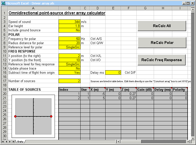
Download Excel spreadsheet (ZIP file, 75KB) This Excel spreadsheet will display polar and frequency response graphs for an array of omnidirectional point-source radiators (for example, subwoofer loudspeakers) in a specified arrangement. The main fields for user entry are shown with yellow backgrounds. The table below with a grey background defines the positions and characteristics of the sources (radiators).
Each source is defined in terms of its position in three axes relative to the origin. The X axis extends to the right, the Y axis extends to the front (towards the bottom of the polar chart), and the Z axis extends upwards. The ground is assumed to be at Z=0. Each source also has a gain value in decibels, a delay in milliseconds, and a polarity control. The sources may be switched on and off using the "Use" column. The number of sources to be used is defined in the "Number of sources" box (cell B17, set to two in the example above). Any sources beyond the number defined that appear within the table are ignored. The small graph to the left of the table of sources gives a pictorial indication of the positions (in X and Y axes only) for all sources within the table. Each "tick" mark represents 1m (i.e. there's 5m in each axis in each direction). The ear height of the listener (i.e. height in the Z axis) should be specified in cell B4. The value given here affects both the polar and frequency response plots. The calculations can optionally include the effects of "ground bounce", i.e. reflections from the plane of the ground at Z=0. This can be switched on or off using the "Include ground bounce" box (cell B5). If ground bounce is switched off here, there's no longer anything special about the plane of Z=0 and other ground bounce options within the spreadsheet are ignored. Polar chart
The frequency for the polar chart is selected in cell B7 and may be swept up and down using Ctrl-A and Ctrl-S. The radius distance for the polar (i.e. the distance from the origin to the listener) is selected in cell B8 and may be swept up and down using Ctrl-Q and Ctrl-W. The reference level for the polar chart is a single driver at unity gain positioned at the origin. However, the reference level may optionally include the "ground bounce" (i.e. reflection from the plane of Z=0, increasing the reference level by 6dB), and this is controlled using cell B9. After making changes, the polar chart should be updated
by clicking the "Recalc Polar" button or by pressing Ctrl-R. Polar levels
The "Polar average" level is the RMS average
around the entire polar. Note that this average is calculated using
the values at the 1 degree resolution employed for the display.
As a result, if the polar contains very sharp nulls, the average value
shown may not be identical to the theoretical calculated value. Frequency response graph
The X and Y positions for the listener (i.e. the position at which the frequency response is calculated) must be specified in cells B11 and B12. The X position (i.e. to the left or right) may be swept up and down using Ctrl-K and Ctrl-L. The Y position (i.e. to the front or back) may be swept up and down using Ctrl-I and Ctrl-O. The Z position of the listener is the ear height specified in cell B4. The reference level for the frequency response graph may be either a single driver at unity gain positioned at the origin, or the first source within the list of sources (including its specified gain). The reference level may optionally include the "ground bounce" (the reflection from the plane of Z=0). The reference level to be used for the frequency response chart is specified in cell B13. The frequency response graph may optionally include a phase trace which is shown in blue. This is enabled using cell B14. The phase values are shown in blue on the right-hand end of the graph. The phase display may be removed from the graph using the "Clear phase trace" button. The "time of flight" between the origin and the listener may optionally be subtracted out, and this is controlled using cell B15. An additional time of flight may be subtracted out (whether or not "Subtract time of flight" is enabled) by specifying the required value in milliseconds in cell E15. This value may be swept up and down in tenths of a millisecond by using Ctrl-D and Ctrl-F. After making changes, the frequency response graph should
be updated by clicking the "Recalc Freq Response" button or
by pressing Ctrl-R. Construct array
The sources are always placed at Y=0 and centred at X=0. The array sits on the ground (above Z=0), and the vertical position of the bottom row of sources is one half of the vertical spacing between drivers. The gain, delay, and polarity values within the list
of sources are not changed by the "Construct array" function.
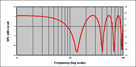
Naturally, the positions generated can be tweaked at will. Examples The example graphs above show two sources spaced apart by 10m (for example, subwoofers on either side of a stage). The polar shows the response at 50Hz at 20m radius, and the frequency response shows the response for a listener 10m in front of the sources at 2m off to the right.
© 2014, 100dB sound |
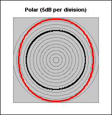
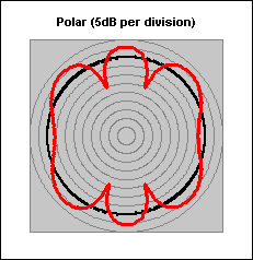 The
polar pattern display resolution is 5dB per annular division, and will
show a minimum value of –40dB. The heavy black line indicates
unity (0dB). The direction of the positive X axis extends towards
the right of the graph and the direction of the positive Y axis extends
towards the bottom of the graph. The chart is drawn with 1 degree
resolution.
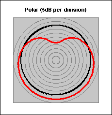
The
polar pattern display resolution is 5dB per annular division, and will
show a minimum value of –40dB. The heavy black line indicates
unity (0dB). The direction of the positive X axis extends towards
the right of the graph and the direction of the positive Y axis extends
towards the bottom of the graph. The chart is drawn with 1 degree
resolution.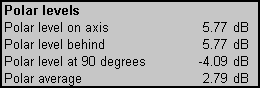 The
"Polar levels" box shows numeric levels at particular points
on the polar chart. "On axis" is towards the bottom of
the chart; "behind" is towards the top, and "90 degrees"
is towards the right.
The
"Polar levels" box shows numeric levels at particular points
on the polar chart. "On axis" is towards the bottom of
the chart; "behind" is towards the top, and "90 degrees"
is towards the right.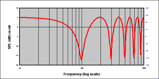 The
frequency response graph shows frequency from 10Hz to 1kHz using a logarithmic
scale, and SPL in decibels relative to the reference value.
The
frequency response graph shows frequency from 10Hz to 1kHz using a logarithmic
scale, and SPL in decibels relative to the reference value.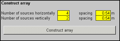 The
"Construct array" box provides a quick way to construct a rectangular
array of sources. Select the number of sources to be created both
horizontally and vertically, the spacing between their centres both horizontally
and vertically, and click the "Construct array" button.
The
"Construct array" box provides a quick way to construct a rectangular
array of sources. Select the number of sources to be created both
horizontally and vertically, the spacing between their centres both horizontally
and vertically, and click the "Construct array" button.